
In the vast tapestry of physics, the spring constant emerges as a thread of resilience and elasticity, weaving together principles of energy conservation and mechanical dynamics. Understanding how to find the spring constant via the lens of energy conservation not only elucidates the behavior of springs but also showcases the profound interconnectedness of physical phenomena. At the heart of this exploration lies a simple yet intriguing experiment that embodies an enduring principle: potential energy morphs into kinetic energy as a spring releases its stored energy.
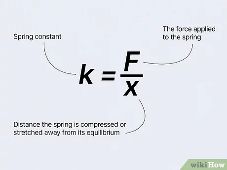
To embark on this journey of discovery, one must first grasp the fundamental concepts underpinning the spring constant, represented by the symbol “k”. This constant quantifies the stiffness of a spring, acting as a coefficient that correlates the force exerted by the spring to its displacement from the equilibrium position. Mathematically, this relationship is encapsulated in Hooke’s Law: F = kx, where F stands for the force applied, k is the spring constant, and x is the displacement.
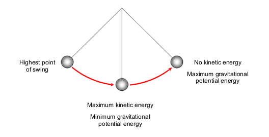
Imagine a spring, poised like a coiled serpent ready to spring into action. When we stretch or compress a spring, we store elastic potential energy, much like the tension in a bowstring. The beauty of this energy lies in its ability to transition seamlessly into kinetic energy when the spring is released. Thus, the conservation of energy principle states that the total energy present in a closed system remains constant; energy can neither be created nor destroyed, only transformed.
The first step in discovering the spring constant entails a hands-on experiment that lays bare the elegance of this transformation. Gather the following materials: a spring with known dimensions, a mass (preferably a set of weights for various increments), a ruler, and a sturdy support to suspend the spring. As you prepare to conduct the experiment, consider this space as a miniature laboratory where the laws of physics will be tested and revealed.
Start by securing the spring vertically, allowing it to hang freely. Attach the mass at the lower end of the spring. As the weight pulls down, the spring will extend, manifesting its elastic properties. Measure the initial displacement from the spring’s equilibrium position when no weight is applied. This point represents the zero-energy state—a zero-sum balance between the potential energy and kinetic energy.
As increments of mass are added, measure the new displacements each time. With each added weight, note the direct correlation between the mass and the resultant extension of the spring. As a rule of thumb, ensure that the spring remains within its elastic limit to avoid permanent deformation, akin to nurturing a fragile ecosystem; moderate changes yield the highest returns.
After you’ve meticulously recorded the data, it’s time to delve deeper. For each weight (mass), calculate the force applied, given by the equation F = mg, where m is the mass and g is the acceleration due to gravity (approximately 9.81 m/s²). Now you have two essential variables: the force exerted (F) and the corresponding displacement (x).
The next step involves plotting these data points on a graph with force (F) on the y-axis and displacement (x) on the x-axis. As you connect the dots, you’ll see a linear relationship beginning to unfold. The slope of this line represents the spring constant (k), providing a tangible measurement of the spring’s stiffness. It’s an enlightening revelation—what begins as mere data transforms into a visual metaphor for stability in a dynamic world.
Once the graph is constructed, utilize the formula for the slope of a line (rise over run) to determine the spring constant: k = ΔF / Δx. Here, ΔF represents the change in force, and Δx represents the change in displacement. This equation embodies the duality of tension and extension, revealing how a spring’s responsiveness mirrors the delicate balance of various systems in nature.
The interplay of energy transformations can further be elucidated by considering the potential energy stored in the spring when displaced. The elastic potential energy (U) can be calculated using the formula: U = 1/2 kx². This encapsulation of energy emphasizes the profound nature of conservation: energy is not lost; it merely exists in different forms, reminding us of the cyclical patterns observed in environmental systems.
Through this experiment, you have interlaced the conceptual fabric of physics with empirical practice. Understanding how to find the spring constant using energy conservation not only enriches your knowledge but also contributes to a greater awareness of the principles governing motion and energy within our universe. Just as springs react to force, so too do all living systems respond to environmental changes, mirroring the delicate equilibrium Earth maintains amidst a backdrop of escalating climate challenges.
In conclusion, the quest to find the spring constant is more than a mere academic exercise; it stands as a metaphor for resilience and adaptability. As humanity grapples with the looming threat of climate change, the lesson from springs serves as a poignant reminder that equilibrium can be achieved through careful observation and calculated actions. By understanding the delicate interactions within our ecosystems, we can harness the lessons of physics to foster innovation, sustainability, and ultimately, a thriving planet for future generations.